A Note on Classical Interest Rate Risk and Risk Management¶

Abstract:

A summary of classical Interest Rate risk and risk management. It is inspired by [Bierwag], [Christensen], [delaGrandville], [Fabozzi], [FabozziKonishi] and wikipedia.

At first it is assumed that there is constant calculation rate $r_0$ for all time periods of length 1, it is a flat yield curve and the discount factors (see `Day count conventions and discount factor functions`_) are $(1+r_0)^{-t_i}$ .

Based on the definition of dateflow_ we now consider dateflows/cashflows as future payments $(c_i)^n_{i=1}$ at times (dates) $(t_i)^n_{i=1}$ . In short this can be written as $(c_{t_i})^n_{i=1}$ or $(c_{t_i})$ .

There are the following standardized dateflow/cashflow types at equally spaced time intervals, ie $(t_i - t_{i-1})^n_{i=2}$ all has the same value:

Zero bond - One future payment consisting of both repayment of dept and rates.

Annuity - Here all future payments are constant. All payments consists of both downpayments and rates. The rate part is exponentially decaying over time.

Bullit - Here all future payments except the last are a constant rate payment. The last payment is a full repayment of dept and a constant rate payment. A Zero bond might be considered as a special case of a Bullit.

Series - Here all future payments has a constant downpayment part and an exponential decaying rate part.

It is worth nothing that for these dateflow/cashflow types all payments are of same sign.

These dateflow/cashflow structures are used to define deposits, bond (being standardized deposit) and different types of swaps.

Present Value, Spread and Risk¶

Now assuming a constant calculation rate $r_0$ for for all time periods of length 1 the Present Value (PV) of a dateflows/cashflows as future payments $(c_{t_i})$ is:

$PV(r_0) = \sum^{n}_{i=1} c_i \cdot (1 + r_0)^{-t_i}$

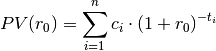
However sometimes it is possible to get a value for the present value (PV) from the market $PV_0$ , eg if a standardized bond is traded.

Then there is a high chance that PV based on the calculation rate differs from the observed market value ( $PV_0$ ).

A reasonable question is which calculation rate leads to the observed market value.

This leads to the following definitions. First a calculation principle:

Definition, Internal Rate:

The Internal Rate (IR) is the calculation rate that makes the calculated present value ( $PV(r_0)$ ) equal to a present value ( $PV_0$ ), ie:

$PV(IR) = PV_0$

It is to be considered as an avarage rate for a cashflow through out the cashflow duration.

Secondly using the calculation principle above (Internal rate) and an observed market value:

Definition, Yield to Maturity or “Mark to Market” Rate:

The Yield to Maturity is the internal rate when the present value is the observed market value, ie:

$PV(IR) = Market value$

Finally using the Internal rate defining the rate at start:

Definition, Par Rate:

A Par Rate is the Internal Rate when a bond is releashed, ie:

$PV(IR) = "100"$

The calculation rate can be set from all kinds of principles, e.g.:

Using a fixed calculation rate

Using yield to maturity

Theorem, Uniqueness of the internal rate

One can make the following observations:

The PV function has a horizontal asymptote $y = 0$

The PV function has a vertical asymptote $r = -1$

And as a special case (All future payments of same sign):

If all future payments are positive (negative) the PV function is

Positive (negative)

Decreasing (increasing)

Convex (concave)

Either way it is a monotonic function and hence there will be a unique solution, ie a unique rate, for each functional value

For a convex (concave) PV function the rate r is negative if and only if it’s function value $PV(r)$ is above (below) the sum of all payments $\sum^{n}_{i=1} c_i$ , ie the rate is 0

Proof:

Since the times $(t_i)^n_{i=1}$ all are positive, $\lim_{r \rightarrow \infty} PV(r) = 0$ , ie the PV function has a horizontal asymptote $y = 0$

Since the times $(t_i)^n_{i=1}$ all are positive, the PV function has a vertical asymptote $r = -1$

Discount factors like $(1 + r)^{-t}$ will always be positive for all $r > -1$ . Note that we are only looking at future times so t is positive. Hence the first order derivative of the discount factor is always negative since:

$\frac{\delta}{\delta r}(1 + r)^{-t} &= -t \cdot (1 + r)^{-t-1} \\ &< 0, \forall r > -1$

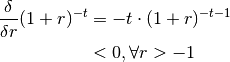
A similar argument shows that the second order derivative is always positive.

So looking at present value function:

$PV(r) = \sum^{n}_{i=1} c_i \cdot (1 + r)^{-t_i}$

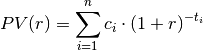
for a dateflows/cashflows as future payments $(c_i)^n_{i=1}$ at times (dates) $(t_i)^n_{i=1}$ it is obvious that the signs of $PV(r)$ and it’s derivatives only are dependent of the signs and sizes of $(c_i)^n_{i=1}$ .

A special case is when all future payments are of the same sign. If all are positive, then the present value will be positive, the first order derivative will be negative and the second order will be positive.

And reverse when all future payments are negative.

In either case the PV function is monotone and hence there is a unique internal rate for each present value.

Since $PV(0) = \sum^{n}_{i=1} c_i$ and the PV function is monotone the last statement is true.

Q.E.D.

So it is easy to find the internal rate when all cash flows are of the same sign. And this way we get a unique Mark To Market rate given a market value.

Evaluation of present value¶

According to some authors the best way to evaluate the present value formula is to use a variant of Horner’s Method:

$PV(r) &= \sum^{n}_{i=1} c_i \cdot (1 + r)^{-t_i} \\ &= ((c_n \cdot r^{t_n -t_{n-1}} + c_{n-1}) \cdot r^{t_{n-1} -t_{n-2}} + c_{n-2}) \cdot ...+ c_1) \cdot r^{t_1}$

The reason for this is that when the times (t) becomes large the discount factors $(1 + r)^{-t}$ becomes close to zero and rounding errors might appear.

In the finance package however it has been chosen to use classical formula for evaluation, ie:

$PV(r) = \sum^{n}_{i=1} c_i \cdot (1 + r)^{-t_i}$

The reason for this is the wish to use vector based calculations throughout the package.

In the package decimalpy a datatype PolyExponents is made to implement the Horner method.

First construct the npv as a function of 1 + r

 >>> from decimal import Decimal
 >>> from decimalpy import Vector, PolyExponents
 >>> cf = Vector(5, 0.1)
 >>> cf[-1] += 1
 >>> cf
 Vector([0.1, 0.1, 0.1, 0.1, 1.1])
 >>> times = Vector(range(0,5)) + 0.783
 >>> times_and_payments = dict(zip(-times, cf))
 >>> npv = PolyExponents(times_and_payments, '(1+r)')
 >>> npv 
 <PolyExponents(   0.1 (1+r)^-0.783
                 + 0.1 (1+r)^-1.783
                 + 0.1 (1+r)^-2.783
                 + 0.1 (1+r)^-3.783
                 + 1.1 (1+r)^-4.783
                 )>

Get the npv at rate 10%, ie 1 + r = 1.1:

>>> OnePlusR = 1.1
>>> npv(OnePlusR)
Decimal('1.020897670129900750434884605')

Now find the internal rate, ie npv = 1 (note that default starting value is 0, which isn’t a good starting point in this case. A far better starting point is 1 which is the second parameter in the call of method inverse):

>>> npv.inverse(1, 1) - 1
Decimal('0.105777770945873634162979715')

So the internal rate is approximately 10.58%

Now let’s add some discount factors, eg reduce with 5% p.a.:

So the discount factors are:

>>> discount = Decimal('1.05') ** - times

And the discounted cashflows are:

>>> disc_npv = npv * discount
>>> disc_npv 
<PolyExponents(
      0.09625178201551631581068644778 x^-0.783
    + 0.09166836382430125315303471217 x^-1.783
    + 0.08730320364219166966955686873 x^-2.783
    + 0.08314590823065873301862558927 x^-3.783
    + 0.8710523719402343459094109352 x^-4.783)>

And the internal rate is:

>>> disc_npv.inverse(1, 1) - 1
Decimal('0.053121686615117746821885443')

And now it is seen that the internal rate is a multiplicative spread:

>>> disc_npv.inverse(1, 1) * Decimal('1.05') - 1
Decimal('0.105777770945873634162979715')

which is the same rate as before.

Duration and Convexity¶

One might want to keep the calculation rate $r_0$ and look at the changes or spread (s) in relation to that: $r_0 + s$ . Hence $r_0$ is the generel or average rate across cashflows whereas the spread (s) is the individual part covering the difference from the average/generel rate in order to become mark to market.

This way the present value calculation becomes:

$PV_{r_0}(s) = \sum^{n}_{i=1} c_i \cdot (1 + r_0 + s)^{-t_i}$

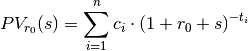
And that is the notation we will use below.

Note

This type of spread is added to rate using bond market discounting.

Definition, Macauley Duration:

The Macauley duration or rather the bond duration as defined below is a weighted average of the payment times using the present values of cashflows as weights (this assumes that the cashflows are of same sign)

$D_{r_0}(0) &= \frac{-(1 + r_0) \cdot \frac{\delta PV_{r_0}(s)}{\delta s}|_{s=0}}{PV_{r_0}(0)} \\ &= \frac{\sum^{n}_{i=1}{t_i \cdot c_i \cdot (1 + r_0)^{-t_i}}}{PV_{r_0}(0)}$

Theorem, Reddingtons immunity

When a rate shock (a parallel shift) is added to the calculation rate then the Macauley Duration is the time before the PV for a cashflow $(c_{t_i})$ is risk free, ie the rate shock is absorbed.

Proof:

We look at the future value at time $t_*$ of the present value $PV_{r_0}(0)$ and examine when the future value $(1 + r_0 + s)^{t_*} \cdot PV_{r_0}(s))$ is risk free regarding rate shocks s, ie:

$(\frac{\delta }{\delta s}\left[(1 + r_0 + s)^{t_*} \cdot PV_{r_0}(s)\right])|_{s=0} &= 0 \\ \Updownarrow \\ (\frac{\delta PV_{r_0}(s)}{\delta s} \cdot (1 + r_0 + s)^{t_*} + t_* \cdot (1 + r_0 + s)^{t_* - 1} \cdot PV_{r_0}(s))|_{s=0} &= 0 \\ \Updownarrow \\ (1 + r_0)^{t_* - 1} \cdot (\frac{\delta PV_{r_0}(s)}{\delta s}|_{s=0} \cdot (1 + r_0) + t_* \cdot PV(0)) &= 0 \\ \Downarrow (PV_{r_0}(0) \neq 0)\\ (1 + r_0)^{t_* - 1} \cdot PV_{r_0}(0) \cdot (-D_{r_0}(0) + t_*) &= 0$

So the future value is risk free when $t_* = D_{r_0}(0)$

Q.E.D.

This result is not that important. It shows that the duration is the time before a (parallel) rate shift/shock is absorbed.

It does not show what happens, when PV is 0 which is a problem eg with interest rate swaps.

And it is irrelevant since it would be better to measure eg the time to illiquidity or the value at risk.

The result is only presented for historical reasons.

A bond is itself a portfolio of zero bonds. Since duration and maturity are equal for zero bonds it follows that duration is subadditive, ie the duration of the portfolio is at most the sum of the durations for the parts of the portfolio.

Theorem, Duration for a portfolio

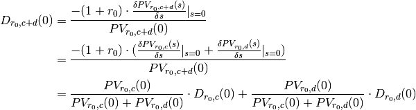
Now the Macauley duration for the sum of two cashflows $(c_{t_i})$ and $(d_{t_i})$ is the present value weighted sum of the durations for each cashflow, ie:

$D_{r_0, c+d}(0) &= \frac{PV_{r_0, c}(0)}{PV_{r_0, c}(0) + PV_{r_0, c}(0)} \cdot D_{r_0, c}(0) + \frac{PV_{r_0, d}(0)}{PV_{r_0, c}(0) + PV_{r_0, d}(0)} \cdot D_{r_0, d}(0)$

An necessary assumption is that all present values $PV_{r_0, c}(0), PV_{r_0, d}(0), PV_{r_0, c+d}(0)$ are nonzero.

Proof:

Now assume two cashflows $(c_{t_i})$ and $(d_{t_i})$ . The present value of the sum of cashflows is the sum of the present values of each cashflow, ie:

$PV_{r_0, c+d}(0) = PV_{r_0, c}(0) + PV_{r_0, d}(0)$

$D_{r_0, c+d}(0) &= \frac{-(1 + r_0) \cdot \frac{\delta PV_{r_0, c+d}(s)}{\delta s}|_{s=0}}{PV_{r_0, c+d}(0)} \\ &= \frac{-(1 + r_0) \cdot (\frac{\delta PV_{r_0, c}(s)}{\delta s}|_{s=0} + \frac{\delta PV_{r_0, d}(s)}{\delta s}|_{s=0})}{PV_{r_0, c+d}(0)} \\ &= \frac{PV_{r_0, c}(0)}{PV_{r_0, c}(0) + PV_{r_0, d}(0)} \cdot D_{r_0, c}(0) + \frac{PV_{r_0, d}(0)}{PV_{r_0, c}(0) + PV_{r_0, d}(0)} \cdot D_{r_0, d}(0)$

Q.E.D.

An similar argument can be made for the modified duration.

This only valid when the PVs $PV_{r_0, c}(0), PV_{r_0, d}(0)$ and their sum $PV_{r_0, c+d}(0)$ are nonzero.

Since there the only elements in the portfolio formula are PVs and durations of each cashflows, the formula can be generalized to when PVs and durations comes from different yieldcurves.

To improve the use of Durations the concept of convexity is introduced.

Definition, Macauley Convexity:

$C_{r_0}(0) &= \frac{(1 + r_0)^2 \cdot \frac{\delta^2 PV_{r_0}(s)}{\delta s^2}|_{s=0}}{PV(0)} \\ &= \frac{\sum^{n}_{i=1}{(t_i+1) \cdot t_i \cdot c_i \cdot (1 + r_0)^{-t_i}}}{PV_{r_0}(0)}$

The rationale for the convexity is following Taylor approximation around s = 0:

$PV_{r_0}(s) &\approx PV_{r_0}(0)\left[1 - \frac{D_{r_0}(0)}{1+r_0} \cdot s + \frac{1}{2} \cdot \frac{C_{r_0}(0)}{(1+r_0)^2} \cdot s^2 \right] \\ & \Downarrow PV_{r_0}(0) \neq 0 \\ \frac{PV_{r_0}(s)}{PV_{r_0}(0)} - 1 &\approx \frac{-D_{r_0}(0)}{1+r_0} \cdot s + \frac{1}{2} \cdot \frac{C_{r_0}(0)}{(1+r_0)^2} \cdot s^2$

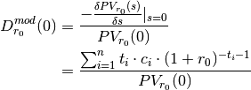
Modified Duration is the elasticy for the present value with regards to to the rate. As can be seen the modified duration is almost the same as the Macauley duration.

Definition, Modified Duration:

$D_{r_0}^{mod}(0) &= \frac{-\frac{\delta PV_{r_0}(s)}{\delta s}|_{s=0}}{PV_{r_0}(0)} \\ &= \frac{\sum^{n}_{i=1}{t_i \cdot c_i \cdot (1 + r_0)^{-t_i - 1}}}{PV_{r_0}(0)}$

And in the modified case it is also possible to define a second order effect, ie a modified convexity.

Definition, Modified Convexity:

$C_{r_0}^{mod}(0) &= \frac{\frac{\delta^2 PV_{r_0}(s)}{\delta s^2}|_{s=0}}{PV_{r_0}(0)} \\ &= \frac{\sum^{n}_{i=1}{(t_i+1) \cdot t_i \cdot c_i \cdot (1 + r_0)^{-t_i - 2}}}{PV_{r_0}(0)}$

To see how modified duration and modified convexity can used to approximate the changes in present value due to rate changes s one has to look at the Taylor approximation of ln(PV):

$\ln(PV_{r_0}(s)) &\approx \ln(PV_{r_0}(0)) - D_{r_0}^{mod}(0) \cdot s + \frac{C_{r_0}^{mod}(0) - D_{r_0}^{mod}(0)^2}{2} \cdot s^2 \\ & \Downarrow PV_{r_0}(0) \neq 0 \\ PV_{r_0}(s) &\approx PV_{r_0}(0) \cdot \exp \left[ - D_{r_0}^{mod}(0) \cdot s + \frac{C_{r_0}^{mod}(0) - D_{r_0}^{mod}(0)^2}{2} \cdot s^2 \right]$

When there is significant curvature/convexity the last approxomation is better. The last approximation does also have a Macauley version:

$PV_{r_0}(s) &\approx PV_{r_0}(0) \cdot \exp \left[ - \frac{D_{r_0}(0)}{1+r_0} \cdot s + \frac{C_{r_0}(0) - D_{r_0}(0)^2}{2 \cdot (1+r_0)^2} \cdot s^2 \right]$

When the present value is zero as might be the case with eg. interest rate swaps other measure are needed.

Below are 2 such measures that tries to handle the problem with zero present values:

Definition, PV01:

Price Value of a 01 (a basis point = 0.0001) is defined as:

$PV01 = (\frac {\partial PV_{r_0}(s)}{\partial s})|_{s=0} \cdot 0.0001$

Definition, PVBP:

Price Value of a Basis Point (= 0.0001) is defined as:

$PVBP = PV_{r_0}(0) - PV_{r_0}(0.0001)$

Using the tangent formula $PV_{r_0}(0.0001) = PV01 + PV_{r_0}(0)$ it is easy to see that the 2 are almost identical (except for the sign).

But here there are no literature suggesting how to handle portfolios. And here is a problem since a basis point might have different probability for different cashflows.

Note

In the Macauley setup presented in most textbooks there is one parameter, the rate, to get a Mark to Market value. This way different cashflows aren’t comparable since they have different rate.

In this presentation the individual rate is split into a common calculation rate $r_0$ and a individual spread s.

This way the Mark to market can be accessed by the spread and portfolio risk can accessed by using risk calculations based on the common rate $r_0$ .

This is a forerunner for the use of yield curves in the risk calculations. One way of seeing the common calculation rate $r_0$ in the next setup is as the constant yield curve.

On the other hand it is obvious that the setup used here contains the classical macauley setup when the common calculation rate is zero, ie $r_0 = 0$

Also it is obvious that the greater spread the less of the market value is explained by the the common calculation rate $r_0$ and hence the greater risk must be associated to such a cashflow.

Fisher-Weil’s Duration and Convexity¶

Fisher-Weil duration is a refinement of Macauley’s duration which takes into account the yield curve, ie the different prices for different future payments.

Fisher-Weil duration is based on the present values of the cashflows instead of just the payments.

The idea is that in a perfect world a yield curve can return the exact value of a future payment and hence a set of future payments, ie a cashflow.

Using a yieldcurve to get the prices means that if there still is a spread different from zero then it must explain something else, eg the incorporated optionality or the credit risk.

In `Addding a Parallel Shift or a spread`_ it is argued that from a mathematical point of view it is better to use a multiplicative spread.

Since the multiplicative spread is more natural using continous forward rates and continous discounting we follow the classical setup we use a yield curve returning the continous forward rate at time t and use continous discounting to get the price.

Definition, Present value, exponential notation:

The Present Value (PV) of a dateflow/cashflow as future payments $(c_{t_i})$ is:

$PV = \sum^{n}_{i=1} c_i \cdot e^{-r_{t_i} \cdot t_i}$

Here the $(r_{t_i})_i$ are the continous forward rates at times $(t_i)_i$

Definition, Multiplicative spread, exponential notation:

The multiplicative spread, s, is a constant added to the continous forward rates. It is an avarage shift that can be used eg for making Mark to market perfect.

Combining the last 2 definitions one gets a formula for the present value of a cashflow, $(c_{t_i})$ , as a function of the multiplicative spread, s:

$PV(s) &= \sum^{n}_{i=1} c_i \cdot e^{-(r_{t_i} + s) \cdot t_i} \\ &= \sum^{n}_{i=1} [c_i \cdot e^{-r_{t_i} \cdot t_i}] \cdot e^{-s \cdot t_i}$

The last derivations shows why the spread is called multiplicative. It is contained in a simple discount factor multiplied to the discounted cashflows.

Note that the spread is similar to the rate in the Uniqueness of the internal rate theorem. So everything said there for the rate goes for the spread as well.

Risk measures from above are defined almost similar as above. Eg we have

Definition, Modified Duration, continous discounting:

$D^{mod}(0) &= \frac{-\frac{\delta PV(s)}{\delta s}|_{s=0}}{PV(0)} \\ &= \frac{\sum^{n}_{i=1}{t_i \cdot [c_i \cdot e^{-r_{t_i} \cdot t_i}]}}{PV(0)}$

The only real problem is how to define Macauley duration and convexity. But here we apply the fact that the multiplicative spread appears as a separate discount factor, so we consider the discounted cashflows by the yieldcurve as the real cashflow. Hence:

Definition, Duration function, continous discounting:

First we define the Duration function:

$D(s) = \frac{-(1 + s) \cdot \frac{\delta PV(s)}{\delta s}}{PV(s)}, PV(s) \neq 0$

And noting that $D(0)$ is both the Macauley and the modified durations (see above). If no yieldcurve is used to discount then $D(r_0)$ is the Macauley duration where $r_0$ is the calculation rate.

And similar:

Definition, Convexity function:

$C(s) = \frac{(1 + s)^2 \cdot \frac{\delta^2 PV(s)}{\delta s^2}}{PV(s)}, PV(s) \neq 0$

Again $C(0)$ is both the Macauley and the modified convexities. And if no yieldcurve is used to discount then $C(r_0)$ is the Macauley convexity where $r_0$ is the calculation rate.

Table Of Contents

This Page

A Note on Classical Interest Rate Risk and Risk Management¶

Present Value, Spread and Risk¶

Evaluation of present value¶

Duration and Convexity¶

Fisher-Weil’s Duration and Convexity¶

Navigation

Table Of Contents

This Page

Quick search

A Note on Classical Interest Rate Risk and Risk Management¶

Present Value, Spread and Risk¶

Evaluation of present value¶

Duration and Convexity¶

Fisher-Weil’s Duration and Convexity¶

Navigation